Abstract Art with ML
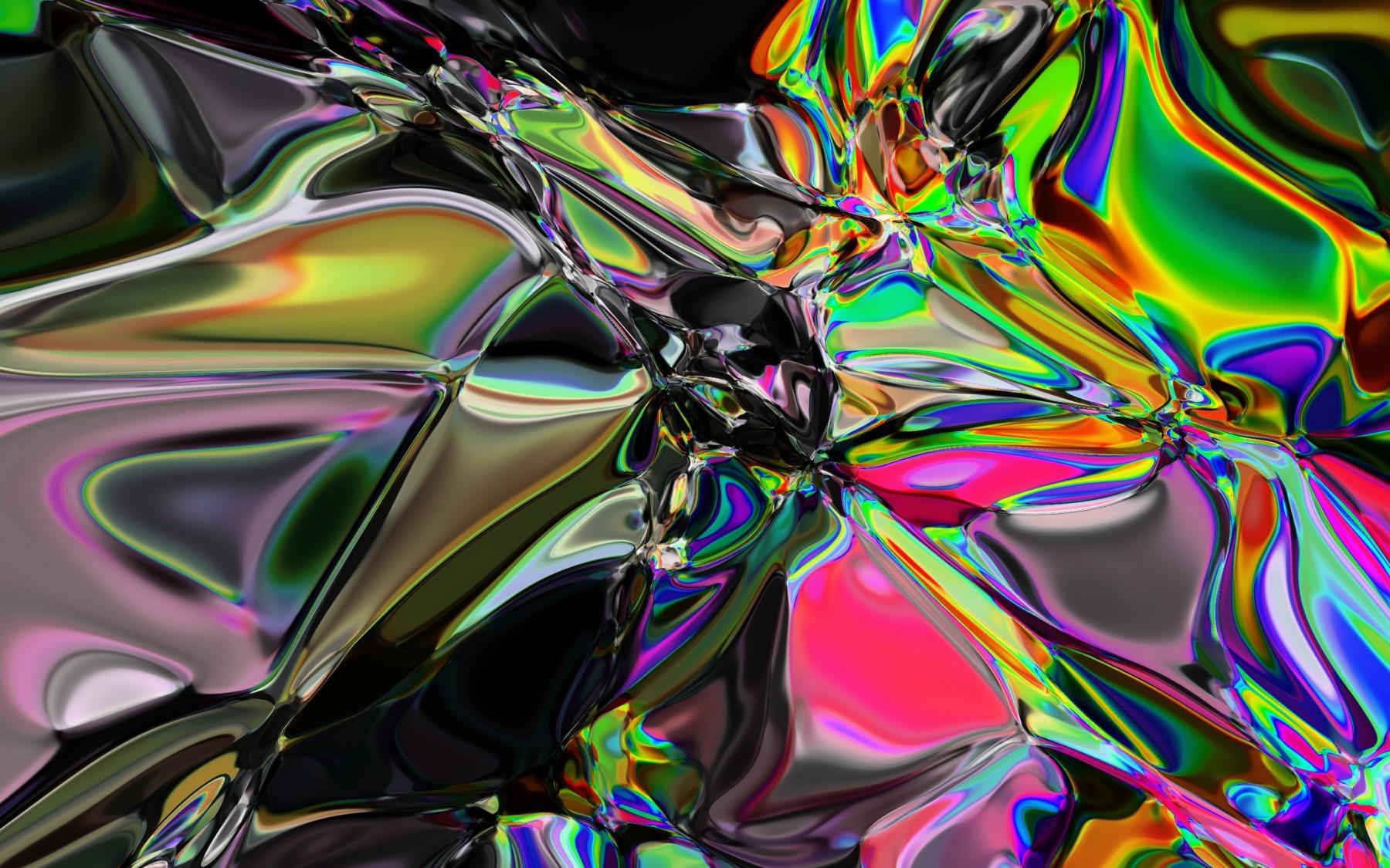
Randomly initialised neural networks are able to produce visually appealing images. In this post, we explore what compositional pattern producing networks are, how they can be parameterised and what kind of images can be obtained using this technique.
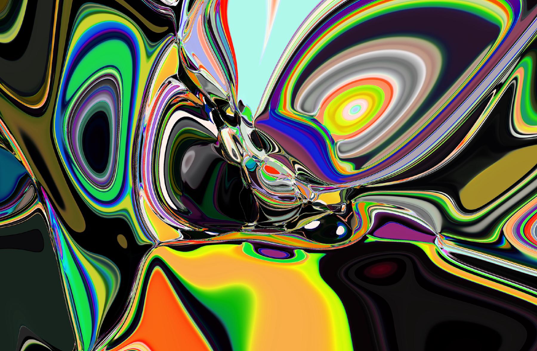
Did you know that randomly initialised neural networks actually produce pretty cool pictures?
This post will be all about generating art with random neural nets. You will be able to generate your own art using a pattern generator that runs in your browser. This means you can experience these networks for yourself. But first, let me explain.
Table of Contents
Compositional Pattern Producing Networks
A compositional pattern producing network, or CPPN in short, is a network, in this case we will mainly focus on neural nets, that given some parameters produces a visual pattern. The main idea here is to slide the network over all the x‑y-coordinates in an image and produce a 3‑channel (rgb) color output for each pixel in the output image. We can look at this network in the following way:
This network, since it’s continuous and differentiable, outputs locally correlated values, meaning, sampling the network on two different very close points will lead to a very similar output value. This basically results in the property that the image we can generate from it, we could call smooth.
Another cool property this has, is that it has “infinite” resolution, because you can just scale the coordinates the network receives as inputs.
Parameters
Now we could simply run the network as it is. And this in fact works. But we take this a little step further by adding certain other inputs to the network with the aim of having the network generate more complex images.
For example we can add the radius and an adjustable parameter . With these modifications our network can be described like the following.
with . The radius not only provides a nice non-linearity but it also enables the network to correlate the output color to the distance to the origin, because points on the same circumference receive the same values for .
While the radius changes with and , the parameter is static over the course of the image. In essence, you can think of this parameter as the z‑parameter. When sampling from the 3‑dimensional cube with parameters , we look at the slice at position .
You can get very creative with these parameters and we’ll explore more exotic configurations later on.
Initialisation
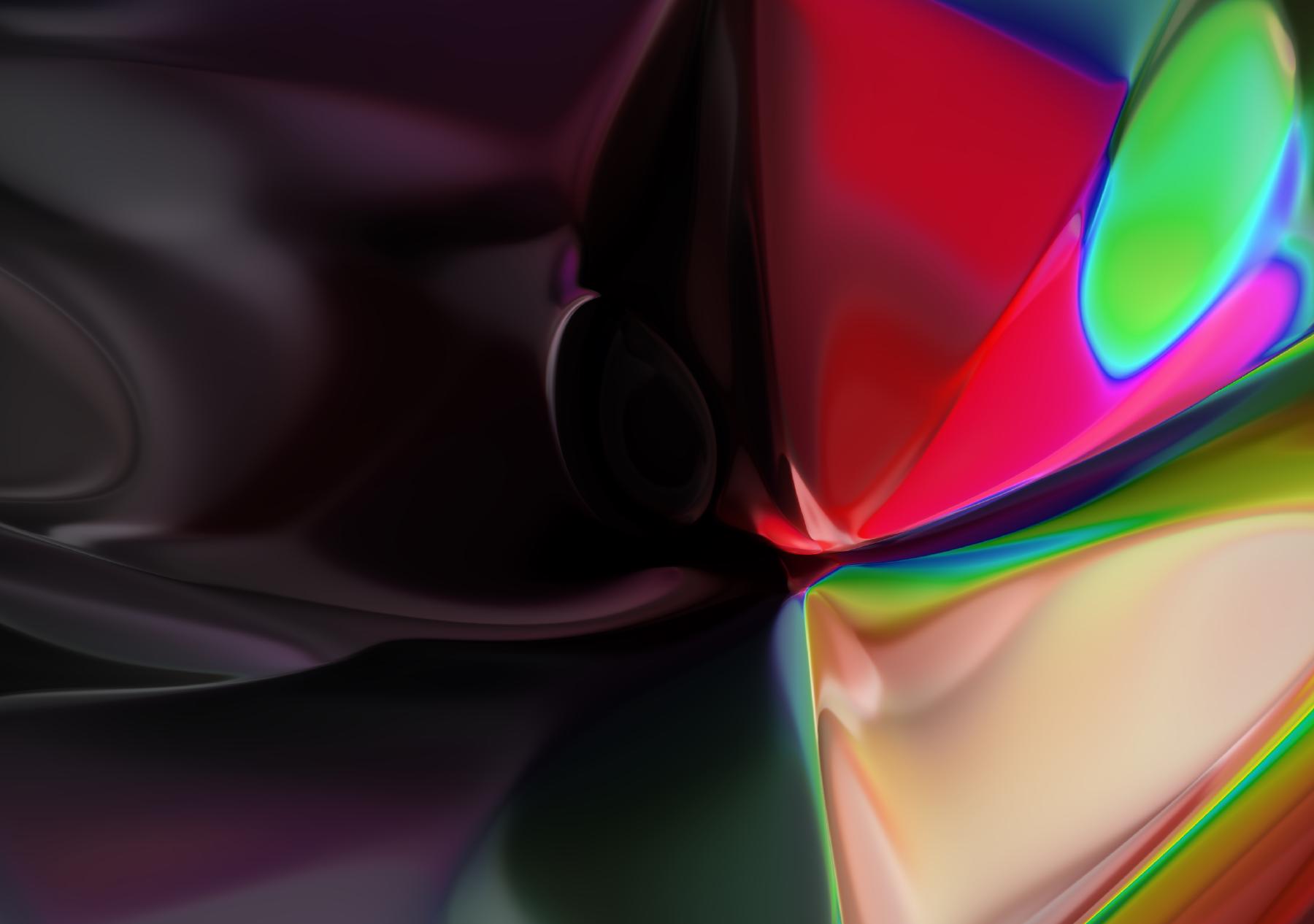
The output of a neural network is defined a) by its inputs which we talked about in the last section and b) by its weights. The weights therefore play a crucial role in how the network behaves and thus what the output image will look like.
In the example images throughout this post, I mainly sampled the weights from a Gaussian distribution with a mean of zero and with a variance dependent on the number of input neurons and a parameter which I could adjust to my taste.
Interactive Generator
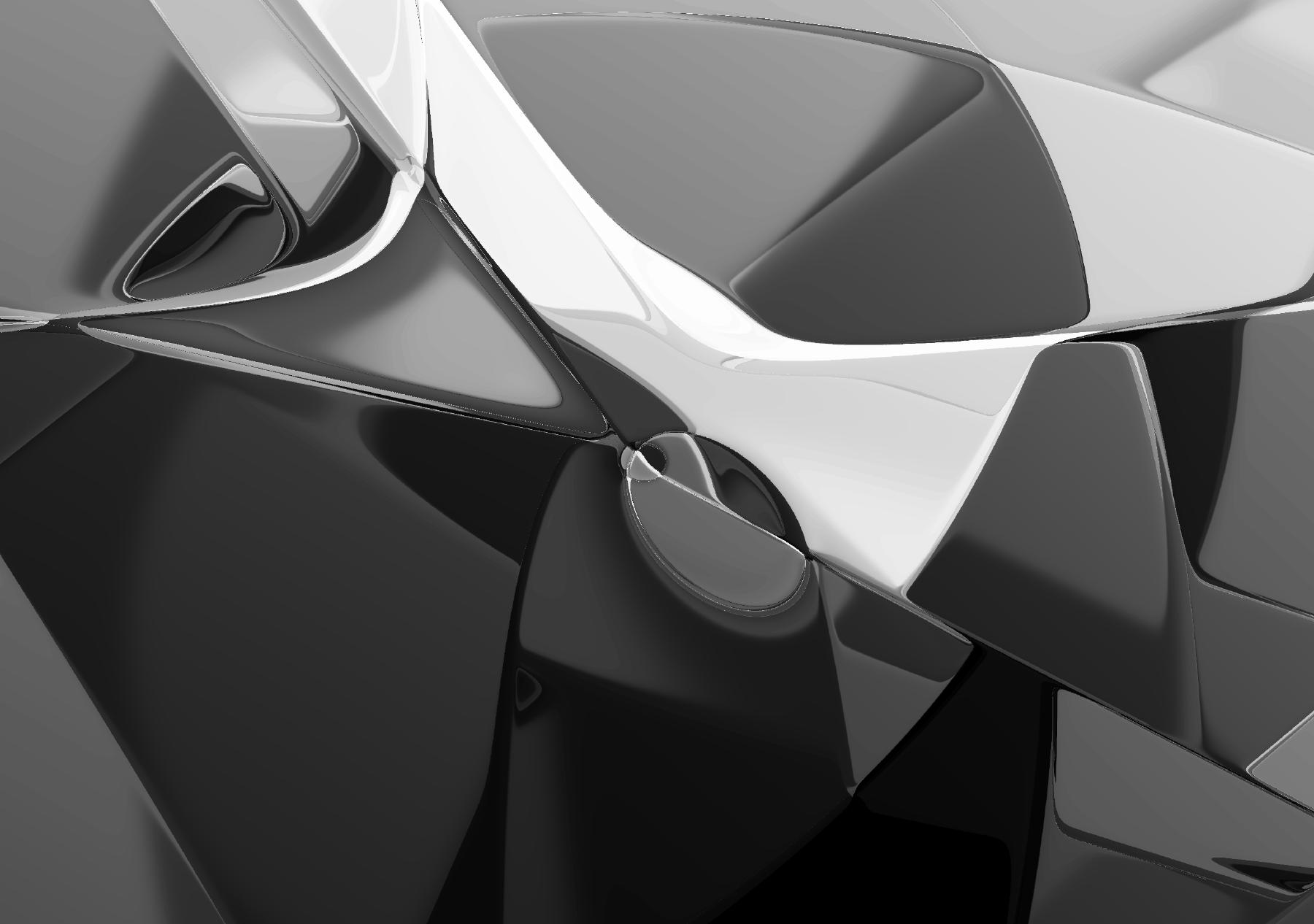
Now to the fun part. Here is a progressive image generator based on the principle of CPPNs. You can adjust the Z‑value and , choose if you want a black and white image and explore the seed space. Note, that the random number generator used for the Gaussian distribution will always produce the same values for the same seed, which is cool, because you can share the seed and retrieve the same result.
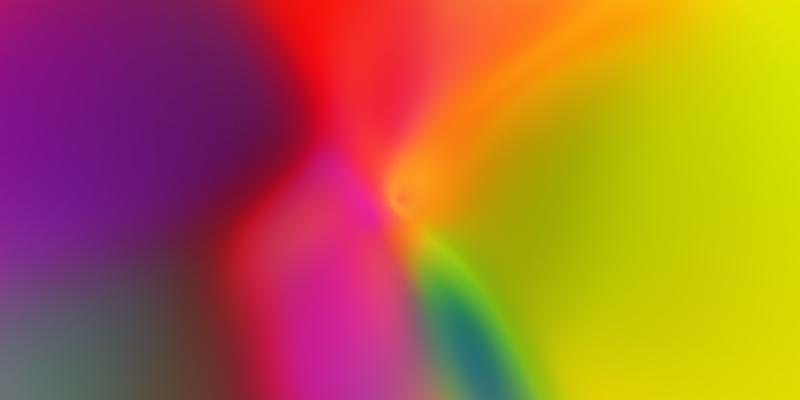
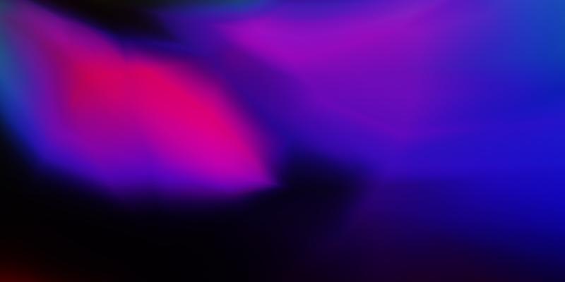
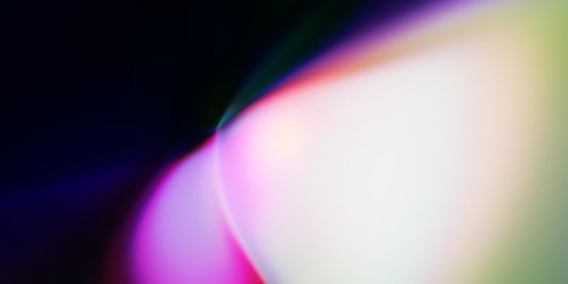
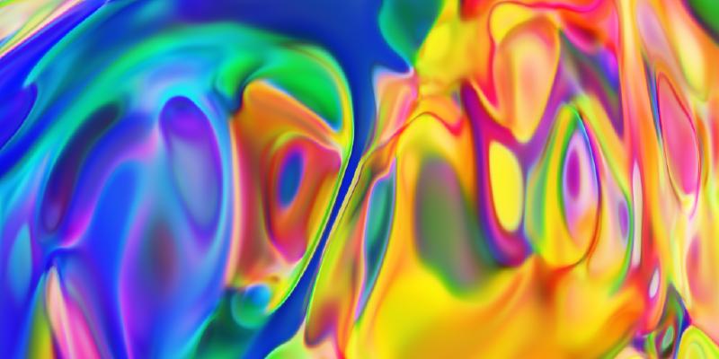
I compiled a list of example seeds that I found compelling while I played with the tool. Try these seeds for the start and then explore the space yourself! :)
And these are just some examples. Try changing the seed, the time or the variance yourself and maybe, just maybe, you come across some masterpiece! 😛
Exploring Exotic Architectures
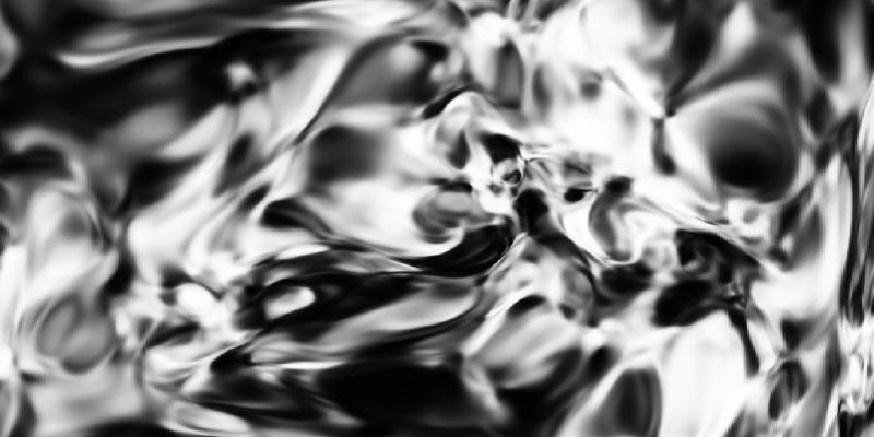
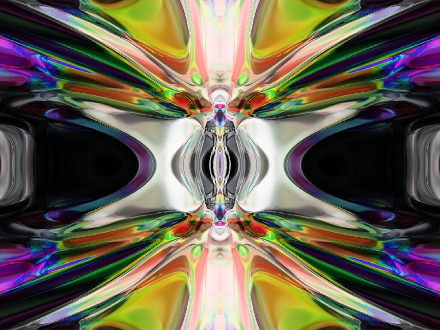
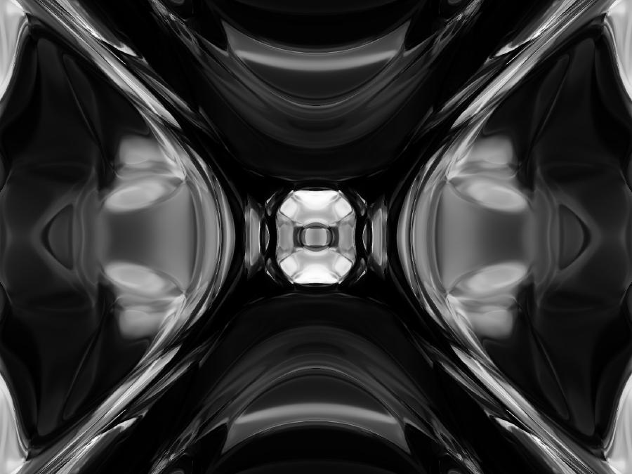
In this section, I want to show you some results I’ve been getting with some more exotic architectures.
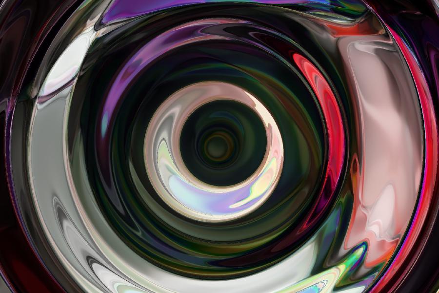
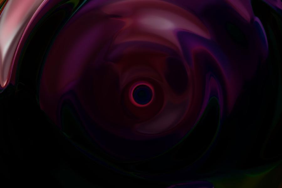
As you can see, these images behave very differently. A single parameter more makes a big difference in the activations of the networks.
Wrapping up
Now that we have gone through several architectures, explored multiple configurations and looked at a bunch of images, it’s time to wrap up. But I want to wrap up by pointing to some possible improvements.
- Train these networks using backpropagation. That’s the obvious one. What’s not obvious, is on what to train it.
- As a follow up to training: one way to supercharge this method of creating art would be to incorporate human feedback e.g. using adversarial networks. For instance, humans could be shown two images which they have to choose the one they prefer from. Then, an adversarial network could learn the probability that a given image is chosen by a human, and use the gradient of this adversarial network for backpropagation on the generator network.
- Also, there are a lot of things I didn’t try. Therefore, one could explore even more of the architecture and parameter space. Changing bias initialisation, kernel initialisation, using different network topologies, or even trying different color spaces.
In terms of use case: these images make great color and gradient inspiration! Also, I just recently replaced my Spotify playlist covers with these. They make pretty great album artworks (don’t they?).
Anyway, that’s it for now. I hope you have enjoyed this blog post. If you did, I’d appreciate if you consider subscribing to my blog via RSS. I’ll try to publish blog posts regularly here. See you then!
I published the code used to generate the images in this post as well as the source code for Figure 4 on GitHub. Python code is based on 1 and runs using Tensorflow. You can find the repository here.